Here’s a problem from Sheldon Axler’s Linear Algebra Done Right (3rd ed), from the chapter regarding “Orthogonal Complements and Minimization Problems”, example 6.58.
This exercise offers an enlightening use of functions as vectors and projections to solve minimization problems, which are of great interest in Calculus and Machine Learning, and even Quantum Computing.
Problem Statement
Find a polynomial u with real coefficients and degree at most 5 that approximates $\sin(x)$ as well as possible on the interval $[-\pi, \pi]$ in the sense that: $$ \int_{-\pi}^{\pi} |\sin(x) - u(x)|^2 \ dx $$ is as small as possible. Compare this to the Taylor Series approximation.
While the book contains a nice explanation of how to solve it, I wanted to take it a step further and implement it in Python. We’ll soon see why you wouldn’t want to do this by hand. The way we’ll solve it is among Linear Algebra’s most coveted concepts: projections.
Solving It Algebraically
This problem brings with it an example of using functions as vectors, a mechanic that some might need a moment to digest. Consider the space of continuous real-valued functions over the interval $[-\pi, \pi]$, which we’ll call $C$. Let’s see how this forms a vector space and how we can take advantage of that.
Checking It’s a Vector Space
To determine if it’s a vector space, we need to check the axioms from LADR 1.19 regarding the elements of the set in question. Suppose we have functions $f, g, z \in C$ and $a \in \mathbb{R}$.
- Since these functions are continuous over a subset of $\mathbb{R}$, we know that $f + g$ and $af$ will produce another continuous function (prop 9.4.9, Analysis 1, Tao), so the set obeys closure under vector addition and scalar multiplication
- We get additive associativity and commutativity inherently from $+$
- Since constant functions are continuous, we can take $g = 0$ as the additive identity and get: $f + g = g + f = f$
- We obtain additive inverses by taking $g = -f$ to get: $f + g = f + (-f) = f-f = 0$
- Continuous functions obey the distributive property when multiplied by scalars in $\mathbb{R}$
Thus $C$ is a vector space. We know that all polynomials are continuous functions over $\mathbb{R}$, and that $\sin(x)$ is a continuous function over $[-\pi, \pi]$; therefore we have $\sin(x)$, polynomials $\in C$.
Defining An Inner Product
An inner product on a vector space is a function that returns a number given two vectors. If we can define a valid inner product, we can say that $C$ is an inner product space.
We’re generally used to the inner product on $\mathbb{R}^n$, the dot product, but if we want to generalize this to functions, we can take the inner product as: $$ \langle f, g \rangle = \int_{-\pi}^{\pi} f(x)g(x) dx $$
I’ll leave it as an exercise to the reader to check this actually defines an inner product, based on the axioms in LADR 6.A.3. Equipping this inner product to $C$ makes it an inner product space, which allows us to compute projections.
Rephrasing The Problem
We know that $\sin(x)$, polynomials $\in C$, so take $v = \sin(x)$ and let $U \subset C$ be a subspace containing all polynomials of at most degree 5.
We can rephrase the problem as follows: we want to find a vector $u \in U$ such that $|v-u|$ is as small as possible.
With this rephrasing, we can solve the problem “quickly”.
Projection As A Service
We make use of two theorems from Linear Algebra; we’ve fulfilled prerequisites by constructing a vector space $C$ and a finite-dimensional subspace $U$. We can define a basis for $U$ as: $$ {1, x, x^2, x^3, x^4, x^5} $$
The theorems we’ll use are as follows:
- Given a finite-dimensional subspace $U \subset C$, the shortest vector from $f \in C$ to $U$ is the orthogonal projection of $f$ onto $U$ (LADR 6.C.56)
- We can compute the orthogonal projection using an orthonormal basis of the subspace (LADR 6.C.55): $$ P(U, f) = \langle f, e_1 \rangle e_1 + \dots + \langle f, e_n \rangle e_n $$
The first theorem tells us that we simply need to compute the projection to get our solution, and the second gives us a way to compute it.
However, we still need an orthonormal basis, and the current basis of $U$ isn’t orthonormal. To be orthonormal, each vector in the basis needs to have length 1 and have an inner product of 0 with every other basis vector.
We can easily see the current basis isn’t orthonormal by considering $\langle 1, 1 \rangle$, which evaluates to $2\pi$ and fails to be normalized, and $\langle 1, x^2 \rangle$, which evaluates to $2\pi^3/3$ and fails to be orthogonal.
To create an orthonormal basis, we use the Gram-Schmidt process on the current basis of $U$. If we define projecting one vector onto another as: $$ \text{proj}_u(v) = \frac{\langle v, u \rangle}{\langle u, u \rangle} u $$
Then the Gram-Schmidt process looks like this:
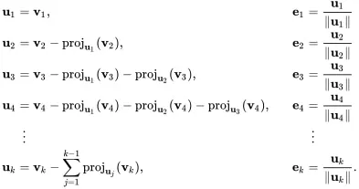
Recall that our inner product is a definite integral, so we can already see that this is going to be a tedious task to solve the question. In our case, $k = 6$ because the subspace $U$ has 6 basis vectors.
Let’s assume we’ve computed the orthonormal basis with the process defined above, obtaining ${e_1 , …, e_6}$, then all we need to do is compute $P(U, \sin(x))$ using the new basis.
Doing so gives you exactly the polynomial that minimizes the difference between it and $\sin(x)$, within the interval $[-\pi, \pi]$. Thus, we’ve theoretically obtained our answer.
Taylor Series Approximation
The last part of the question asks us to compare our approximation to the Taylor Series approximation of $\sin(x)$, up to degree 5. The Taylor Series is: $$ \sin(x) = x - \frac{x^3}{3!} + \frac{x^5}{5!} $$
and the computation produces this graph ($\sin(x)$ (blue), the Taylor Series approximation (red), $x = \plusmn \ \pi$ (green)):
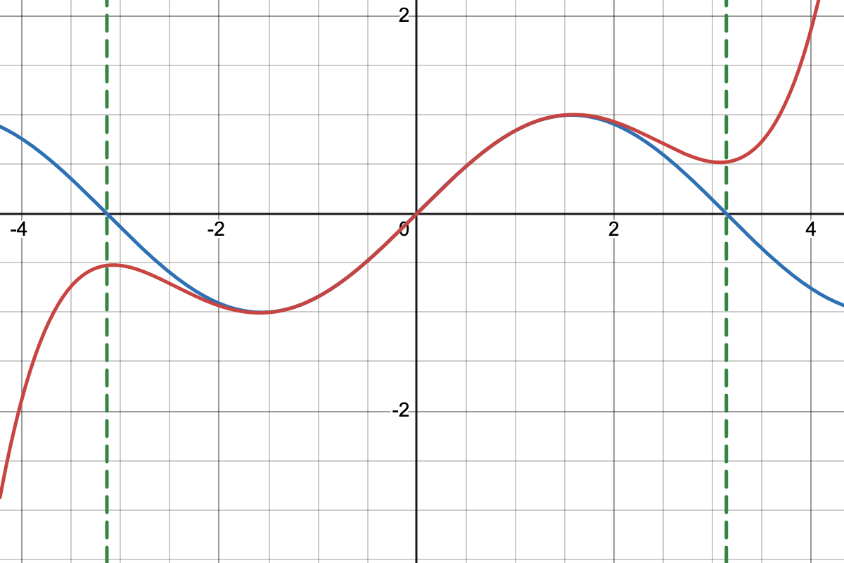
We see that even before getting to x = ± 2, the approximation begins to fail and gets worse really quickly.
Computing The Approximation In Python
To compute the approximation, we can use the Python library SymPy. SymPy is a library for symbolic computations, essentially a Computer Algebra System (CAS).
We’ll start with the preamble of the script, containing constants and imports:
from sympy import (
    integrate,
    pi,
    sin,
    sqrt,
    Symbol,
)

I = [-pi, pi]
Note: SymPy is for symbolic computations, meaning we need to pass a Symbol to each function so that the system performs computations properly. This explains the s which appears as a parameter in the functions below.
Inner Product
Let’s start by implementing the inner product we defined before. Recall that it’s simply a definite integral, which we can write as so:
def inner_product(f, g, s):
  return integrate(f * g, (s, I[0], I[1]))
Length
To compute length, we use the fact that: $$ |v| = \sqrt{\langle v, v \rangle} $$
def length(f, s):
  return sqrt(inner_product(f, f, s))
Gram-Schmidt
We’ll implement the version of Gram Schmidt that we defined above, though there are other ways to implement it computationally. The benefit in implementing it this way will be the correspondence between the code and the theory we discussed before.
def gram_schmidt(basis, s):
  e = dict()

  # The first one is easy, we only have one term
  e[1] = basis[0] / length(basis[0], s)

  # For computing the rest of the orthonormal basis vectors
  for i in range(1, len(basis)):
      e[i+1] = basis[i]
      for k in range(1, i):
          e[i+1] -= inner_product(basis[i], e[k], s) * e[k]
      e[i+1] *= 1/length(e[i+1], s)
  return e
Orthogonal Projection
Finally, we prepare the orthogonal projection function, which will actually compute the final projection onto the subspace we’re interested in:
def orthogonal_projection(v, basis, s):
    dim = len(basis)
    p = inner_product(v, basis[1], s)
    for i in range(2, dim+1):
        p += inner_product(v, basis[i], s) * basis[i]
    return p
Final Computation
We’re finally ready to put the computations together:
def main():
    x = Symbol("x")
    basis = [x ** i for i in range(6)]
    orthonormal_basis = gram_schmidt(basis, x)
    op = orthogonal_projection(sin(x), orthonormal_basis, x)
    return op.evalf()

if __name__=="__main__":
    result = main()
    print(result)
Note that the final call of op.evalf() converts the exact answer coefficients to decimals for a more readable expression.
The answer we get is:
0.00564311797634678*x**5 - 0.155271410633428*x**3 + 0.987862135574673*x
which, rounded to the sixth decimal point, is the same as the result from LADR!
Let’s graph the result (black) in Desmos on top of the original approximation:
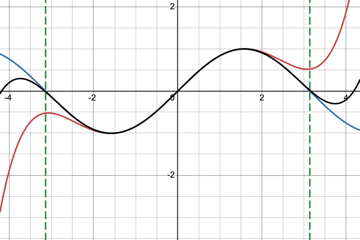
We see that the polynomial approximation does much better than the Taylor Series approximation in the interval $[-\pi, \pi]$.
Final Thoughts
Through this problem, we got to explore both the power of Linear Algebra, and the power of SymPy for symbolic computations. You can explore further by trying different intervals and continuous functions, or try to approximate with different degrees of polynomials.
Notice how we didn’t even have to consider the original integral we needed to minimize. We were able to translate the theory from Linear Algebra into a concrete script that gave us a quick solution, and there’s still room for optimization! There’s a reason this branch of math underpins so many quantitative fields.